Table-of-Contents
- Requirements
- Quick start
- Troubleshooting
- How to use it in your project
- Contributing
- Technical description
- Authors
- Publications
- Acknowledgments
- Third-party tools
Requirements ⇧
‘Future Weather Generator’ needs at least JAVA SE 17.
Quick start ⇧
- After installing or updating Java to the latest version, download the ‘Future Weather Generator’ into the desired applications folder.
- Create a folder where the app will save future weather-generated files.
- Open the app by:
- Double-click the icon or right-click it and open it with Java Launcher.
- In the terminal (Command Line in Windows), change the directory to the app folder and run
‘java -jar FutureWeatherGenerator.java’.
- An initial window will open (Fig. 1), and two actions are available:
- ‘Generate EPW file’ (Fig. 2) prompts the user to provide an EPW file and the output folder to save the morphed files (step 2). The app will create the morphed files for all scenarios and timeframes for the selected general circulation model (GCM) or the ensemble. In addition, the app will save the GCM variables for interpolated location as CSV files and compare each morphed EPW with the original EPW file.
- ‘Compare EPW files’ (Fig. 3) compares two EPW files and saves the comparison CSV files in a given output folder (step 2).
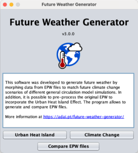
Two options are available: ‘Generate EPW file’ and ‘Compare EPW files’
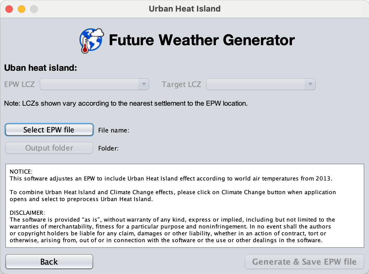
The user can modify EPW files to account for the urban heat island effect. They must choose the LCZ representative of the EPW’s location and the target LCZ. The LCZs shown relate to the nearest settlement to the EPW’s location.
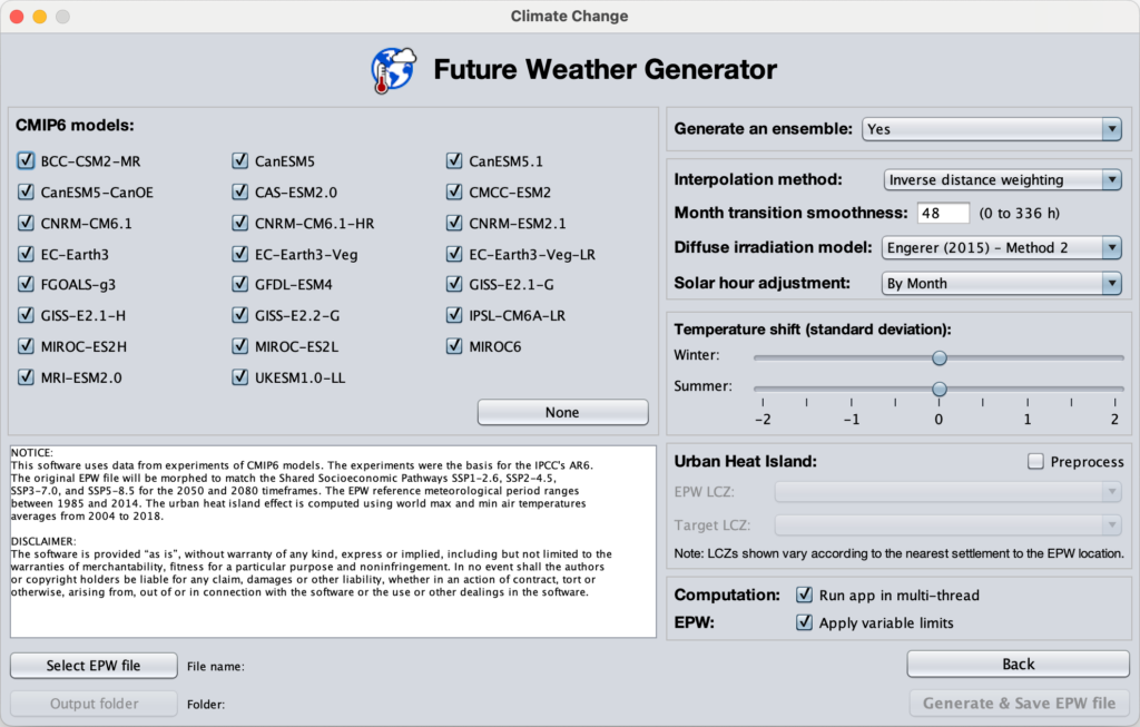
The user can select one or more GCM models and decide whether to create an ensemble. To select the GCMs that best fit the EPW’s region, we recommend using the GCMEval tool (https://gcmeval.met.no). The user can select a different diffuse irradiation model (Ridley, Boland & Lauret, 2010; Engerer, 2015; or Paulescu & Blaga, 2019) and opt for solar hour adjustment (ByMonth or ByDay) or None. The user may also set the hours for a smooth transition at the beginning and end of each month (not applicable to the beginning of January and to the end of December). The app runs in multi-threaded mode by default.
Note: If you have an antivirus software installed, this software might prevent the app from saving the CSV files. In order to overcome this issue, you may pause the antivirus software or add 'Future Weather Generator' to the exception rules.
How to use it in your project ⇧
Run it without GUI in the Terminal (Command Prompt)
You may want to run ‘Future Weather Generator’ from the terminal. In this case, first change to the app folder.
cd %future_weather_generator_folder%The field %future_weather_generator_folder% is the path to the folder where you have the ‘Future Weather Generator’. Then, you can just run the following line to understand which arguments you can use (or see this page for more details).
java -jar FutureWeatherGenerator_v4.0.1.jar -helpYou can create a batch script in MS Windows to morph EPW files recursively inside a folder (save a copy of Future Weather Generator inside as well):
@ECHO OFF

for /r %%F in (*.epw) do (
	java -jar FutureWeatherGenerator_v4.0.1.jar -epw=%%F
)
If you use Linux or macOS, you can use this bash script:
#!/usr/bin/env bash

walk_dir () {
    shopt -s nullglob dotglob

    for FILENAME in "$1"/*; do
        if [ -d "$FILENAME" ]
        then
            walk_dir "$FILENAME"
        else
            if [[ "$FILENAME" == *"epw"* ]]
            then
                DIRECTORY="$(dirname "$FILENAME")/"
                java -cp FutureWeatherGenerator_v4.0.1.jar -epw=$FILENAME
            fi
        fi
    done
}

CURRENT_DIR=.

walk_dir "$CURRENT_DIR"
As a library
You may add the downloaded ‘FutureWeatherGenerator.jar’ to your project as a library. In this case, you only need to save it to your ‘lib’ folder in the project folder and specify it in the classpath.
As source code
In this case, you may download the project folder with the source code from the Bitbucket repository.
Examples
The first example is generating all SSP for all timeframes from any GCM model. The first step is to import the needed classes:
import futureweathergenerator.epw.EPW;
import futureweathergenerator.models.ClimateModel;
After, we load the EPW file in our class or method (uppercase variables PATH_TO_EPW_FILE, PATH_TO_OUTPUT_FOLDER, and others are paths to files and folders):
// Loads original EPW file
EPW epw = new EPW(new StringBuffer(), PATH_TO_EPW_FILE, EPW_VARIABLE_LIMITS, true);
Then, we can add one or all of the GCM models available to generate all future weather EPW files for all timeframes and scenarios:
// Generates all EPW files and CSV files for all SSP and timeframes
// Set the grid point option (GRID_POINT_OPTION):
// 0 - weighted distance of the four nearest points
// 1 - average of the four nearest points
// 2 - nearest point of the four nearest points
// You can specify the number of CPU threads (NUMBER_OF_CPU_THREADS)
// Month transition smoothness (NUMBER_OF_HOURS_FOR_MONTH_TRANSITION_SMOOTHNESS)
// Apply EPW dictionary variable limits (EPW_VARIABLE_LIMITS)
// 0 - No
// 1 - Yes
// Ask to save the output files (DO_NOT_SAVE_OUTPUT_FILES)
// true - does not save the files
// false - saves outputs

// Example for EC-Earth3
ClimateModel model_ec_earth3 = new ClimateModel(
            EC-Earth3,
            null,
            epw,
            PATH_OUTPUT_FOLDER);
model_ec_earth3.readModelGrid();
model_ec_earth3.readModelData(NUMBER_OF_CPU_THREADS, GRID_POINT_OPTION);
model_ec_earth3.generate(
            DO_NOT_SAVE_OUTPUT_FILES,
            EPW_VARIABLE_LIMITS,
            NUMBER_OF_HOURS_FOR_MONTH_TRANSITION_SMOOTHNESS);


// Example for CNRM-CM6-1-HR
ClimateModel model_cnrm_cm6_1_hr = new ClimateModel(
            CNRM-CM6-1-HR,
            null,
            epw,
            PATH_OUTPUT_FOLDER);
model_cnrm_cm6_1_hr.readModelGrid();
model_cnrm_cm6_1_hr.readModelData(NUMBER_OF_CPU_THREADS, GRID_POINT_OPTION);
model_cnrm_cm6_1_hr.generate(
            DO_NOT_SAVE_OUTPUT_FILES,
            EPW_VARIABLE_LIMITS,
            NUMBER_OF_HOURS_FOR_MONTH_TRANSITION_SMOOTHNESS);
You may wish to create an ensemble with those two models.
// Create a list for climate models
List<ClimateModel> list_of_models = new ArrayList<>();

// Add models to the list
list_of_models.add(model_ec_earth3);
list_of_models.add(model_cnrm_cm6_1_hr);

// Create the ensemble
ClimateModel model_ensemble = createEnsemble(models);

// Generate the data
model_ensemble.generate(
            DO_NOT_SAVE_OUTPUT_FILES,
            EPW_VARIABLE_LIMITS,
            NUMBER_OF_HOURS_FOR_MONTH_TRANSITION_SMOOTHNESS);
Referencing and acknowledging
Do not forget to add the following text to your acknowledgments:
We thank the developers of the 'Future Weather Generator' and its funding institutions for making the app free and open to the public. [%your software name%] took advantage of the 'Future Weather Generator' software [https://future-weather-generator.adai.pt/].
If you use ‘Future Weather Generator’ in your studies, please add the following reference:
Rodrigues E, Carvalho D, Fernandes MS, Future Weather Generator – Morphs current weather for performance simulation of buildings in the future. Association for the Development of Industrial Aerodynamics, Coimbra, 2022. URL: https://future-weather-generator.adai.pt/
Or reference our publication:
Rodrigues E, Fernandes MS, Carvalho D, Future weather generator for building performance research: An open-source morphing tool and an application. Building and Environment, 2023; 233:110104. doi:10.1016/j.buildenv.2023.110104.
Contributing ⇧
Reporting issues
Before reporting issues, please update to the latest ‘Future Weather Generator’ version. If the issue persists, check if the bug was already reported in the Bitbucket repository. If the issue has not yet been reported, please provide the following information:
- Operating system
- Java version
- The version of the ‘Future Weather Generator’
- Description of the issue
- Provide all the data needed to reproduce the problem
Suggesting enhancements
Before suggesting an enhancement, please confirm that the proposed enhancement is not already implemented. If such enhancement has not yet been implemented, provide us with a detailed description and include as many details as possible by creating an issue in the Bitbucket repository. Fill in the following template:
- Summary of the enhancement
- Motivation
- Describe alternatives
- Additional context
Code of conduct
The ‘Future Weather Generator’ community comprises a mixture of researchers and volunteers from all over the world, working on every aspect of the distribution, from coding to marketing. Diversity is one of our enormous strengths but can lead to communication issues and unhappiness. To that end, we have a few ground rules that we ask people to adhere to when they’re using project resources. This code of conduct isn’t an exhaustive list of things you can’t do. Instead, take it in the spirit it’s intended – a guide to make it easier to be excellent to each other.
- Be considerate. Other people will use your work, and you, in turn, will depend on the work of others. Therefore, any decision you take will affect users and colleagues, and you should consider those consequences when making decisions.
- Be respectful. Not all of us will always agree, but disagreement is no excuse for poor behavior and manners. We might all experience some frustration now and then. Still, we cannot allow that frustration to become personal attacks. It’s important to remember that a community where people feel uncomfortable or threatened is not productive. Members of the ‘Future Weather Generator’ community should be respectful when dealing with other contributors and people outside the ‘Future Weather Generator’ community and with users of ‘Future Weather Generator.’
When we disagree, we try to understand why. Social and technical disagreements happen all the time, and ‘Future Weather Generator’ is no exception. We must resolve disagreements and differing views constructively. Remember that we’re different. The strength of ‘Future Weather Generator’ comes from its varied community, people from various backgrounds. Different people have different perspectives on issues. Being unable to understand why someone holds a viewpoint doesn’t mean they’re wrong. Don’t forget that it is human to err. Therefore, blaming each other doesn’t get us anywhere. Rather, we offer to help resolve issues and learn from mistakes.
Credits for the sources and inspiration of this Code of Conduct go to the Fedora Project.
Technical description ⇧
The ‘Future Weather Generator’ utilizes results from twenty general circulation models (GCM) environmental variables to morph current local weather data in the format of EPW files into future scenarios and timeframes.
GCM models
The app uses data from the following GCMs models: BCC-CSM2-MR, CanESM5, CanESM5.1, CanESM5-CanOE, CAS-ESM2.0, CMCC-ESM2, CNRM-CM6.1, CNRM-CM6.1-HR, CNRM-ESM2.1, EC-Earth3, EC-Earth3-Veg, EC-Earth3-Veg-LR, FGOALS-g3, GFDL-ESM4, GISS-E2.1-G, GISS-E2.1-H, GISS-E2.2-G, IPSL-CM6A-LR, MIROC-ES2H, MIROC-ES2L, MIROC6, MRI-ESM2.0, and UKESM1.0-LL. The experiments of these models contributed to the 6th IPCC Assessment Report (2022).
Climatic data were retrieved for the present-day climate and two future climate periods:
- For the present-day climate, the reference year 2000 is related to the period between 1985 and 2014.
- For the two future climates, the reference years are 2050 (2036-2065) and 2080 (2066-2095).
Since version 3.0.0, the mean and standard deviation of the differences between baseline and future timeframes of thirty months have been computed.
The app implements four Shared Socioeconomic Pathways (SSP) from the CMIP6:
SSP1-2.6: Global CO2 emissions are cut severely, reaching net zero after 2050. Temperatures stabilize around 1.8 °C higher by the end of the century.
SSP2-4.5: Global CO2 emissions will not reach net zero by 2100. Temperatures will rise by 2.7 °C by the end of the century.
SSP3-7.0: Global CO2 emissions will roughly double from current levels by 2100. By the end of the century, average temperatures have risen by 3.6 °C.
SSP5-8.5: Current CO2 emissions levels will roughly double by 2050. By 2100, the average global temperature will increase to 4.4 °C.
Morphing
The morphing procedure follows Jentsch (2012) general approach based on Belcher et al. (2005). The GCM variables used in the app are the monthly near-surface air temperatures (TAS, TASMAX, and TASMIN), precipitation (PR), near-surface specific humidity (HUSS), air pressure at mean sea level (PSL), total cloud cover percentage (CLT), surface downwelling shortwave radiation (RSDS), snow depth (SND), and near-surface wind speed (SFCWIND). However, this app differs when selecting the GCM grid point. First, the four nearest points to the EPW location in the GCM grid are selected. Then, it averages them into a fifth point corresponding to the cell center. Finally, the app determines the nearest point of those five points in the morphing calculations.
Those GCM variables are used to ‘shift’ and ‘stretch’ several EPW fields, such as ‘N6 Dry Bulb Temperature, ‘N8 Relative Humidity’, ‘N9 Atmospheric Pressure’, ‘N13 Global Horizontal Radiation’, ‘N15 Diffuse Horizontal Radiation’, ‘N21 Wind Speed’, ‘N22 Total Sky Cover’, ‘N30 Snow Depth’, and ‘N33 Liquid Precipitation Depth’. The remaining EPW fields are derived from those morphed fields and calculated using the solar geometry equations (CIBSE, 2002), the Perez et al. (1990) tables, the Kasten et al. (2000) optical air mass table, Ridley et al. (2010) diffuse horizontal radiation calculations, and the ASHRAE Handbook Fundamentals (2017). The fields ‘N20 Wind Direction’, ‘N26 Present Weather Observation’, ‘N27 Present Weather Code’, and ‘N34 Liquid Precipitation Quantity’ are kept the same as in the original EPW file, while the remaining fields are set to missing values.
The monthly ground temperatures at different depths are calculated according to the procedure described in Jentsch (2012), which follows Kusuda and Achenbach (1965) and Lawrie (2003) equations. Lastly, the typical/extreme periods are calculated from the morphed ‘N6 Dry Bulb Temperature’.
N6 Dry Bulb Temperature (°C)
The future ‘N6 Dry Bulb Temperature’ is morphed by first determining a scaling factor ($\alpha t_m$) for the month $m$
$$ \alpha t_m = {{\Delta TASMAX_m – \Delta TASMIN_m} \over {\langle d\dot{b}t_{max} \rangle_m – \langle d\dot{b}t_{min} \rangle_m} } $$
where $\Delta TASMAX_m$ is the GCM change in the average daily maximum dry bulb temperature, $\Delta TASMIN_m$ is the GCM change in the average daily minimum dry bulb temperature, $\langle d\dot{b}t_{max} \rangle_m$ is the average daily maximum dry bulb temperature, and $\langle d\dot{b}t_{min} \rangle_m$ is the average daily minimum dry bulb temperature from the EPW file for the month $m$.
The future ‘N6 Dry Bulb Temperature’ ($dbt$) is then calculated by
$$ dbt = d\dot{b}t + \Delta TAS_m + \alpha t_m \cdot \big(d\dot{b}t – \langle d\dot{b}t \rangle_m \big) $$
where $d\dot{b}t$ is the present ‘N6 Dry Bulb Temperature’ in the EPW file, $\Delta TAS_m$ is the GCM change in the mean dry bulb temperature, and $\langle d\dot{b}t \rangle_m$ is the mean of the present ‘N6 Dry Bulb Temperature’ in the EPW file for the month $m$.
N7 Dew Point Temperature (°C)
The future ‘N7 Dew Point Temperature’ is determined by using the morphed specific humidity.
First, the future specific humidity ($\gamma$) is calculated by adding the GCM change in mean specific humidity for the month $m$ ($\Delta HUSS_m$) to the present day specific humidity ($\dot{\gamma}$)
$$ \gamma = \dot{\gamma} + \Delta HUSS_m $$
where $\dot{\gamma}$ depends on the present day humidity ratio ($\dot{W}$)
$$ \dot{\gamma} = {\dot{W} \over 1 + \dot{W}} $$
$\dot{W}$ is a function of the present ‘N6 Dry Bulb Temperature’ ($d\dot{b}t$), the present ‘N8 Relative Humidity’ ($r\dot{h}u$), and the present ‘N9 Atmospheric Pressure’ ($a\dot{t}p$), all from the EPW file
$$ \dot{W} = 0.621945 \cdot { r\dot{h}u \cdot \dot{p}’_{ws} |_{dbt, p_{at}} \over a\dot{t}p – r\dot{h}u \cdot \dot{p}’_{ws} |_{dbt, p_{at}}} $$
where $\dot{p}’_{ws}$ is the present saturation pressure of water vapor in the absence of air at a given temperature numerically equal to the considered dry bulb temperature of the air, with $|_{dbt, p_{at}}$ representing a given dry bulb temperature and atmospheric pressure.
Then, the future partial pressure of water vapor ($p_w$) is determined by
$$ p_w = {atp \cdot W \over 0.621945 – W} $$
where $atp$ is the future ‘N9 Atmospheric Pressure’ and $W$ is the future humidity ratio
$$ W = {\gamma \over 1 – \gamma} $$
The future ‘N7 Dew Point Temperature’ ($dpt$) can now be calculated by inverting the equation giving water vapor pressure at saturation from temperature ($p’_{ws}$), using the Newton-Raphson method (iterative) on the logarithm of $p’_{ws}$
$$ dpt = dpt_{iter} – {\ln(p’_{ws} |_{dpt, p_{at}}) – \ln(p_w) \over {d \over dT} \big(\ln(p’_{ws} |_{dpt , p_{at}})\big)} $$
until $dpt$ converges to the value obtained in the previous iteration ($dpt_{iter}$), and where $|_{dpt , p_{at}}$ represents a given dew point temperature (equal to $dpt_{iter}$ in each iteration) and atmospheric pressure.
N8 Relative Humidity (%)
The app uses specific humidity change ($\Delta HUSS$) to calculate the future ‘N8 Relative Humidity’.
First, the future specific humidity ($\gamma$) is calculated by adding the GCM change in mean specific humidity for the month $m$ ($\Delta HUSS_m$) to the present day specific humidity ($\dot{\gamma}$)
$$ \gamma = \dot{\gamma} + \Delta HUSS_m $$
where $\dot{\gamma}$ depends on the present day humidity ratio ($\dot{W}$)
$$ \dot{\gamma} = {\dot{W} \over 1 + \dot{W}} $$
$\dot{W}$ is a function of the present ‘N6 Dry Bulb Temperature’ ($d\dot{b}t$), the present ‘N8 Relative Humidity’ ($r\dot{h}u$), and the present ‘N9 Atmospheric Pressure’ ($a\dot{t}p$), all from the EPW file
$$ \dot{W} = 0.621945 \cdot { r\dot{h}u \cdot \dot{p}’_{ws} |_{dbt, p_{at}} \over a\dot{t}p – r\dot{h}u \cdot \dot{p}’_{ws} |_{dbt, p_{at}} } $$
where $\dot{p}’_{ws}$ is the present saturation pressure of water vapor in the absence of air at a given temperature numerically equal to the considered dry bulb temperature of the air, with $|_{dbt, p_{at}}$ representing a given dry bulb temperature and atmospheric pressure.
Then, the future partial pressure of water vapor ($p_w$) is determined by
$$ p_w = {atp \cdot W \over 0.621945 – W} $$
where $atp$ is the future ‘N9 Atmospheric Pressure’ and $W$ is the future humidity ratio
$$ W = {\gamma \over 1 – \gamma} $$
The future ‘N8 Relative Humidity’ ($rhu$) is then determined by
$$ rhu = {p_w \over p’_{ws} |_{dbt, p_{at}}} $$
where $p’_{ws}$ represents the saturation pressure of water vapor in the absence of air at a given temperature numerically equal to the considered dry bulb temperature of the air ($dbt$), with $|_{dbt, p_{at}}$ representing a given dry bulb temperature and atmospheric pressure.
N9 Atmospheric Pressure (Pa)
The future ‘N9 Atmospheric Pressure’ ($atp$) is determined by adding the GCM change in mean atmospheric pressure at sea level for the month $m$ ($\Delta PSL_m$) to the present ‘N9 Atmospheric Pressure’ from the EPW file ($a\dot{t}p$)
$$ atp = a\dot{t}p + \Delta PSL_m $$
N10 Extraterrestrial Horizontal Radiation (Wh/m2)
First, the day angle ($d’$) for the Julian day ($d$) is determined by
$$ d’ = {{2 \cdot \pi \cdot (d-1)} \over {365}} $$
which allows us to use the equation of time ($EOT$).
$$ EOT = {{ \big( -7.659 \cdot \sin(d’) + 9.863 \cdot \sin(2 \cdot d’ + 3.5932) \big) } \over {60}} $$
The solar time ($SOT$) can then be determined from the local standard time ($LST$), longitude from the EPW location ($\lambda$), and longitude of the time zone from the EPW location ($\lambda_R$)
$$ SOT = LST + {{(\lambda – \lambda_R)} \over {15}} + EOT $$
and calculate the hour angle ($\omega$)
$$ \omega = {{360} \over {24}} \cdot (SOT – 12) $$
which is used to determine Earth’s declination ($\delta$).
$$ \begin{split} \delta = & 0.006918 \\&- 0.399912 \cdot \cos(d’) + 0.070257 \cdot \sin(d’) \\&- 0.006758 \cdot \cos(2 \cdot d’) + 0.000907 \cdot \sin(2 \cdot d’) \\&- 0.002697 \cdot \cos(3 \cdot d’) + 0.00148 \cdot \sin(3 \cdot d’) \end{split} $$
All these are used to calculate the solar altitude angle ($\gamma_s$) using the sine rule.
$$ \sin(\gamma_s) = \sin(\phi) \cdot \sin(\delta) + \cos(\phi) \cdot \cos(\delta) \cdot \cos(\omega) $$
Finally, future ‘N10 Extraterrestrial Horizontal Radiation’ ($ehr$) is calculated by
$$ ehr = \sin(\gamma_s) \cdot edn $$
for all hours with incident solar radiation; and where $edn$ is the future ‘N11 Extraterrestrial Direct Normal Radiation’, presented below.
N11 Extraterrestrial Direct Normal Radiation (Wh/m2)
The future ‘N11 Extraterrestrial Direct Normal Radiation’ ($edn$) is calculated by multiplying the correction factor for the varying solar distance to Earth by the solar constant (1367 W/m2)
$$ edn = 1367 \cdot \big(1 + 0.03344 \cdot \cos(d’) \big)$$
for all hours with incident solar radiation.
N12 Horizontal Infrared Radiation from the Sky (Wh/m2)
First, the atmospheric emissivity ($\varepsilon_{at}$) is determined using future ‘N22 Total Sky Cover’ ($tsc$), future ‘N6 Dry Bulb Temperature’ ($dbt$), and future partial pressure of water vapor ($p_w$).
$$ \varepsilon_{at} = {tsc \over 10} + \Big( 1 – {tsc \over 10} \Big) \cdot 1.24 \cdot \Big( {p_w \over dbt} \Big)^{1/7} $$
In this equation, the future partial pressure of water vapor ($p_w$) is determined by
$$ p_w = rhu \cdot p’_{ws} |_{dbt, p_{at}} $$
where $p’_{ws}$ is the saturation pressure of water vapor in the absence of air at a given temperature numerically equal to the considered dry bulb temperature of the air, $rhu$ is the future ‘N8 Relative Humidity’, and $|_{dbt, p_{at}}$ represents a given dry bulb temperature and atmospheric pressure.
Lastly, future ‘N12 Horizontal Infrared Radiation from the Sky’ ($hir$) is calculated by multiplying the atmospheric emissivity ($\varepsilon_{at}$) by the Stefan-Boltzmann constant ($5.67 \cdot 10^{-8}$) by the future ‘N6 Dry Bulb Temperature’ ($dbt$).
$$ hir = \varepsilon_{at} \cdot 5.67 \cdot 10^{-8} \cdot dbt^4 $$
N13 Global Horizontal Radiation (Wh/m2)
First, the scaling factor for downward surface shortwave flux ($\alpha I_m$) is determined
$$ \alpha I_m = 1 + \Bigg( {{\Delta RSDS_m} \over{\langle g\dot{h}r \rangle_m} } \Bigg) $$
where $\Delta RSDS_m$ is the GCM change of the mean downward surface shortwave flux and $\langle g\dot{h}r \rangle_m$ is the average of the present ‘N13 Global Horizontal Radiation’ ($g\dot{h}r$) for the month $m$.
Lastly, the future ‘N14 Global horizontal Radiation’ ($ghr$) is calculated by multiplying $\alpha I_m$ by the present ‘N14 Global horizontal Radiation’ ($g\dot{h}r$).
$$ ghr = \alpha I_m \cdot g\dot{h}r $$
N14 Direct Normal Radiation (Wh/m2)
The future ‘N14 Direct Normal Radiation’ ($dnr$) is calculated from the solar altitude angle ($\gamma_s$) using the sine rule, the future ‘N13 Global Horizontal Radiation’ ($ghr$), and the future ‘N15 Diffuse Horizontal Radiation’ ($dhr$).
$$ dnr = { {ghr – dhr} \over { sin(\gamma_s) } } $$
N15 Diffuse Horizontal Radiation (Wh/m2)
Paulescu & Blaga (2019)
To describe.
Engerer (2015) – Method 3
To describe.
Ridley, Boland & Lauret (2010)
First, the hourly clearness index ($KT_h$) is determined by dividing the future ‘N13 Global Horizontal Radiation’ ($ghr_h$) by the future ‘N10 Extraterrestrial Horizontal Radiation’ for the hour $h$.
$$ KT_h = { ghr_h \over ehr_h } $$
Similarly, the daily clearness index ($KT_d$) is calculated for designated day $d$.
$$ KT_d = { {\sum_{h=1}^{24} ghr_h} \over {\sum_{h=1}^{24} ehr_h} } $$
According to sunset and sunrise time $h$, the clearness index persistence is determined ($\psi$) for the following cases.
$$ \psi = \begin{cases} \displaystyle {{KT_{h-1} + KT_{h+1}} \over {2}}& \text{sunrise} < h < \text{sunset} \\ \displaystyle KT_{h+1} & h=\text{sunrise} \\ \displaystyle KT_{h-1} & h=\text{sunset} \end{cases} $$
Lastly, the future ‘N15 Diffuse Horizontal Radiation’ ($dhr$) is calculated by
$$ dhr = ghr \cdot {{1} \over { 1 + \exp(-5.38 + 6.63 \cdot KT_h + 0.006 \cdot SOT – 0.007 \cdot \gamma_s + 1.75 \cdot KT_d + 1.31 \cdot \psi) }} $$
using solar time ($SOT$) and solar altitude angle ($\gamma_s$).
N16 Global Horizontal Illuminance (lux)
First, the solar zenith angle ($\theta_s$), precipitable water content ($PWC$), atmospheric brightness ($atb$), and atmospheric clearness ($atc$) are determined from the solar altitude angle ($\gamma_s$), the future ‘N7 Dew Point Temperature’ ($dpt$), the relative optical air mass ($m$) obtained from Table 2 in Kasten and Young (1989), the future ‘N15 Diffuse Horizontal Radiation’ ($dhr$), the future ‘N11 Extraterrestrial Direct Normal Radiation’ ($edn$), and the future ‘N14 Direct Normal Radiation’ ($dnr$).
$$ \theta_s = 90 – \gamma_s $$
$$ PWC = \exp(0.07 \cdot dpt – 0.075) $$
$$ atb = dhr \cdot {m \over edn} $$
$$ atc = {{{{dhr + dnr} \over dhr} + 1.041 \cdot \theta_s^3} \over {1 + 1.041 \cdot \theta_s^3}} $$
With the atmospheric clearness ($atc$), a sky clearness category is obtained to determine the coefficients ($a_i$, $b_i$, $c_i$, and $d_i$) from Table 1 — ‘Discrete Sky Clearness Categories’ and Table 4 — ‘Global Luminous Efficacy’ in Perez et al. (1990), which allow calculating the future ‘N16 Global Horizontal Illuminance’ ($ghi$) according to the following equation
$$ ghi = ghr \cdot \big(a_i + b_i \cdot PWC + c_i \cdot \cos(\theta_s) + d_i \cdot \ln(atb)\big) $$
where $ghr$ is the future ‘N13 Global Horizontal Radiation’.
N17 Direct Normal Illuminance (lux)
To calculate the future ‘N17 Direct Normal Illuminance’ ($dni$) the coefficients ($a_i$, $b_i$, $c_i$, and $d_i$) are obtained from Table 4 — ‘Direct Luminous Efficacy’ in Perez et al. (1990) and used in the following equation
$$ dni = dnr \cdot \big( a_i + b_i \cdot PWC + c_i \cdot \exp(5.73 \cdot \theta_s – 5) + d_i \cdot atb \big), dni \geq 0$$
where $dnr$ is the future ‘N14 Direct Normal Radiation’.
N18 Diffuse Horizontal Illuminance (lux)
In the case of the future ‘N18 Diffuse Horizontal Illuminance’, the coefficients ($a_i$, $b_i$, $c_i$, and $d_i$) are obtained from Table 4 — ‘Diffuse Luminous Efficacy’ in Perez et al. (1990) and used in the following equation
$$ dhi = dhr \cdot \big( a_i + b_i \cdot PWC + c_i \cdot \cos(\theta_s) + d_i \cdot \ln(atb) \big) $$
where $dhr$ is the future ‘N15 Diffuse Horizontal Radiation’.
N19 Zenith Luminance (Cd/m2)
In the case of the future ‘N19 Zenith Luminance’, the coefficients ($a_i$, $b_i$, $c_i$, and $d_i$) are obtained from Table 4 — ‘Zenith Luminance Prediction’ in Perez et al. (1990) and used in the following equation
$$ zlu = dhr \cdot \big( a_i + b_i \cdot \cos(\theta_s) + c_i \cdot \exp(-3 \cdot \theta_s) + d_i \cdot atb \big) $$
where $dhr$ is the future ‘N15 Diffuse Horizontal Radiation’.
N20 Wind Direction (˚)
The future ‘N20 Wind Direction’ is equal to the present ‘N20 Wind Direction’.
N21 Wind Speed (m/s)
For morphing the future ‘N21 Wind Speed’ ($win$), the present ‘N21 Wind Speed’ ($w\dot{i}n$) is multiplied by the GCM relative mean change in wind speed ($WIND_m$) for the month $m$
$$ win = w\dot{i}n \cdot SFCWIND_m$$
N22 Total Sky Cover (deca)
The future ‘N22 Total Sky Cover’ ($tsc$) is calculated by
$$ tsc = {10 \cdot t\dot{s}c + {\Delta CTL_m} \over {10} }, 0 \leq tsc \leq 10 $$
where $t\dot{s}c$ is the present ‘N22 Total Sky Cover’ in the EPW file and $\Delta CTL_m$ is the GCM change of the mean total cloud in longwave radiation for the month $m$.
N23 Opaque Sky Cover (deca)
The future ‘N23 Opaque Sky Cover’ ($osc$) is determined by
$$ osc = { { tsc \cdot o\dot{s}c } \over {t\dot{s}c} }, 0 \leq osc \leq 10 $$
where $tsc$ is the future ‘N22 Total Sky Cover’, $o\dot{s}c$ is the present ‘N23 Opaque Sky Cover’ in the EPW file, and $t\dot{s}c$ is the present ‘N23 Opaque Sky Cover’ in the EPW file.
N24 to N25
These are set to missing values.
N26 Present Weather Observation
The future ‘N26 Present Weather Observation’ is equal to the present ‘N26 Present Weather Observation’.
N27 Present Weather Code
The future ‘N27 Present Weather Code’ equals the present ‘N27 Present Weather Code’.
N28 to N29
These are set to missing values.
N30 Snow Depth (cm)
The present ‘N30 Snow Depth’ ($s\dot{n}d$) is multiplied by the GCM relative mean change in snow depth ($SND_m$) for the month $m$
$$snd = s\dot{n}d \cdot SND_m$$
N31 to N32
These are set to missing values.
N33 Liquid Precipitation Depth (mm)
For morphing the future ‘N33 Liquid Precipitation Depth’ ($pre$), the present ‘N33 Liquid Precipitation Depth’ ($p\dot{r}e$) is multiplied by the GCM relative mean change in precipitation ($PR_m$) for the month $m$
$$pre = p\dot{r}e \cdot PR_m$$
N34 Liquid Precipitation Quantity (h)
The future ‘N34 Liquid Precipitation Quantity’ is equal to the present ‘N34 Liquid Precipitation Quantity’.
Ground Temperatures
The EPW file requires a set of 12-month values for three ground temperature depths (0.5 m, 2 m, and 4 m). In order to determine the monthly ground temperature at a given depth, the ground temperature for each Julian day $d$ must be calculated before averaging each month’s daily ground temperatures. The daily ground temperature ($gt_d$) can be determined with the following equations
$$ x = \sqrt{ {{\pi } \over {D_s \cdot 365} } } \cdot depth $$
$$ y = {{exp(-x)^2 – 2 \cdot exp(-x) \cdot \cos(x) + 1} \over {2 \cdot x^2}} $$
$$ z = { {1 – exp(-x) \cdot \big(cos(x) + sin(x) \big)} \over {1 – exp(-x) \cdot \big(cos(x) – sin(x) \big)} } $$
$$ gt_d = \langle dbt_a \rangle – {{\langle dbt_{amp} \rangle} \over 2} \cdot \cos\Big(2 \cdot \Big({\pi \over 365}\Big) \cdot d – \big(d_{shift} \cdot 0.017214 + 0.341787 \big) – \arctan(z) \Big) \cdot \sqrt{y} $$
where $D_s$ is the thermal diffusivity of the ground (0.055741824 $m^2/day$), $depth$ is the ground depth, $\langle dbt_a \rangle$ is the annual average of the future ‘N6 Dry Bulb Temperature’, $\langle dbt_{amp} \rangle$ is the amplitude of the warmest and coldest future average monthly ‘N6 Dry Bulb Temperature’, and $d_{shift}$ is median day of the month containing the minimum surface temperature $d_{shift} \in \{15, 46, 74, 95, 135, 166, 196, 227, 258, 288, 319, 349 \}$.
Typical/Extreme Periods
Six typical and extreme periods are calculated from the morphed ‘N6 Dry Bulb Temperature’. The typical periods correspond to the week of each season (Winter, Spring, Summer, and Autumn) and present the average temperature closest to that season’s average. The extreme periods are calculated for summer and winter, corresponding to the week with the highest positive and negative differences in the average season temperature.
Table of Fields
The following table presents the EPW’s data fields morphed, calculated, kept the same, and set missing. It also lists required fields on known software using EPW data.
EPW data field | Future Weather Generator | EnergyPlus | epw2wea (Radiance) | clm (ESP-r) |
|---|---|---|---|---|
| N6 Dry Bulb Temperature | ◼︎ | ▲ | ▲ | |
| N7 Dew Point Temperature | ◼︎ | ▲ | ||
| N8 Relative Humidity | ◼︎ | ▲ | ▲ | |
| N9 Atmospheric Pressure | ◼︎ | ▲ | ||
| N10 Extraterrestrial Horizontal Radiation | ◼︎ | |||
| N11 Extraterrestrial Direct Normal Radiation | ◼︎ | |||
| N12 Horizontal Infrared Radiation from the Sky | ◼︎ | ▲ | ||
| N13 Global Horizontal Radiation | ◼︎ | |||
| N14 Direct Normal Radiation | ◼︎ | ▲ | ▲ | ▲ |
| N15 Diffuse Horizontal Radiation | ◼︎ | ▲ | ▲ | ▲ |
| N16 Global Horizontal Illuminance | ◼︎ | |||
| N17 Direct Normal Illuminance | ◼︎ | |||
| N18 Diffuse Horizontal Illuminance | ◼︎ | |||
| N19 Zenith Luminance | ◼︎ | |||
| N20 Wind Direction | ◼︎ | ▲ | ▲ | |
| N21 Wind Speed | ◼︎ | ▲ | ▲ | |
| N22 Total Sky Cover | ◼︎ | ▲ | ||
| N23 Opaque Sky Cover | ◼︎ | ▲ | ||
| N24 Visibility | ◻︎ | |||
| N25 Ceiling Height | ◻︎ | |||
| N26 Present Weather Observation | ◼︎ | ▲ | ||
| N27 Present Weather Codes | ◼︎ | ▲ | ||
| N28 Precipitable Water | ◻︎ | |||
| N29 Aerosol Optical Depth | ◻︎ | |||
| N30 Snow Depth | ◼︎ | ▲ | ||
| N31 Days Since Last Snowfall | ◻︎ | |||
| N32 Albedo | ◻︎ | |||
| N33 Liquid Precipitation Depth | ◼︎ | ▲ | ||
| N34 Liquid Precipitation Quantity | ◼︎ | |||
| Ground Temperatures | ◼︎ | ▲ | ||
| Typical/Extreme Periods | ◼︎ | ▲ |
◼︎ – Morphed value
◼︎ – Calculated value
◼︎ – Kept the original value
◻︎ – Set as missing
▲ – Used variable
References
- ASHRAE Handbook – Fundamentals, 2017.
- Belcher S, Hacker J, Powell D. Constructing design weather data for future climates. Build Serv Eng Res Technol 2005;26:49–61. https://doi.org/10.1191/0143624405bt112oa.
- CIBSE Guide J – Weather, solar and illuminance data, 2002.
- Jentsch MF. Climate Change Weather File Generators: Technical reference manual for the CCWeatherGen and CCWorldWeatherGen tools. Southampton: University of Southampton; 2012.
- Kasten F, Young AT. Revised optical air mass tables and approximation formula. Appl Opt 1989;28:4735. https://doi.org/10.1364/AO.28.004735.
- Lawrie LK, EnergyPlus Weather Converter, Subroutine for ground temperature calculation: CalcGroundTemps.f90, Fortran code, 2003.
- Kusuda T, Achenbach PR. Earth temperature and thermal diffusivity at selected stations in the United States. 1965.
- Perez R, Ineichen P, Seals R, Michalsky J, Stewart R. Modeling daylight availability and irradiance components from direct and global irradiance. Solar Energy 1990;44:271–89. https://doi.org/10.1016/0038-092X(90)90055-H.
- Ridley B, Boland J, Lauret P. Modelling of diffuse solar fraction with multiple predictors. Renew Energy 2010;35:478–83. https://doi.org/10.1016/j.renene.2009.07.018.
- Engerer, N. A. Minute resolution estimates of the diffuse fraction of global irradiance for southeastern Australia. Sol. Energy 2015;116:215–237.
- Paulescu, E. & Blaga, R. A simple and reliable empirical model with two predictors for estimating 1-minute diffuse fraction. Sol. Energy 2019; 180:75–84.
Authors ⇧


For those who wish to contribute to the app development, you may report issues in the source code webpage or even ask to be part of the developing team.
Acknowledgments ⇧
This work is framed under the ‘Energy for Sustainability Initiative‘ of the University of Coimbra. The authors are grateful to all Ph.D. students who have tested the app.
We acknowledge the World Climate Research Programme, which, through its Working Group on Coupled Modeling, coordinated and promoted CMIP5, CMIP6, and CORDEX. We thank the climate modeling groups for producing and making available their model output, the Earth System Grid Federation (ESGF) for archiving the data and providing access, and the multiple funding agencies who support CMIP5, CMIP6, CORDEX, and ESGF.
Third-party tools ⇧
- pyfwg – Daniel Sánchez-García’s python wrapper for Future Weather Generator (GitHub and Documentation). It is a robust, step-by-step Python workflow manager.